Announcing a new blogging website, Page Fault

After nearly five years (and nearly 10 years since I started blogging), I’m starting a new blog, Page Fault, at https://www.neilbickford.com/blog/. The first new article is a tutorial that shows you how to build a real-time denoiser in JSFX, REAPER’s audio programming language. It has some nice behavior, and it’s been used in production for several videos at the UCLA Game Music Ensemble.

You’ll also notice that the last two posts have been copied over to Page Fault. Since there are many websites that link to https://nbickford.wordpress.com, this blog will also remain online to avoid breaking those hyperlinks. Please note that some articles on this website are down for maintenance at the moment.

Hyperbolic Self-Similarity

This texture shrinks on one axis while stretching on the other – and yet somehow loops every three seconds.

Here’s the full code of a (very) heavily modified version, which fits in one and a half tweets (you can also view it on Shadertoy):

#define p exp2(fract(iDate.w/3.)+float(i))
void mainImage( out vec4 fragColor, in vec2 fragCoord ){
  for(int i=-9;i<9;i++){
    fragColor+=min(p,1./p)*texture2D(iChannel0,fragCoord*.004*vec2(1./p,p))/3.;
  }
}

Interferometry and the Very Large Array

Congratulations! You’ve just been hired to record the crowd at the Super Bowl!

The producer wants you to figure out how loud each section, and ideally how loud each fan, is cheering so that they can better choose where to station the T-shirt cannons. They don’t want to know the actual dialogue – they’re not the NSA – only each fan’s loudness, or amplitude*. You don’t even have to record the fans’ cheering over time, but just how loud each one is, on average, over the full game.

*technically, loudness is a psychoacoustic property of the amplitude, the average intensity, and the frequency spectrum of the signal, but in this article we’re assuming (for the purposes of keeping it relatively short) that they’re essentially the same.

The only problem?

You’re on the other side of the field, 160 feet away from the nearest spectator. And you have one microphone with which to record all twenty thousand fans.

Source: Getty Images

Hi! This is an introduction to astronomical interferometry and radio telescopy! This article might assume that you have some familiarity with Fourier transforms, but that’s about it. This article is currently in beta; if you find any issues, errors, or omissions, please let me know through the comments below. Thanks!

Algorithms for Threes and 2048

Threes is a terrifically simple, yet tremendously intriguing game from the creative team at Sirvo (Asher Vollmer, Greg Wohlwend, and Big Giant Circles) known for their work on indie games such as Puzzlejuice and Ridiculous Fishing.

The rules are very simple: every time you swipe across the screen, all of the tiles try to move in the direction you swiped. Two tiles can combine if their values add up to 3, or if the tiles are equal and both integer multiples of 3. If you try to combine two tiles (by squishing one against the wall) and they can’t, then they act as a barrier, and that particular column or row doesn’t budge. Finally, there’s the part which makes it tricky: Every time you move the tiles, another tile is introduced. The goal is to reach the elusive 6144 tile, or more realistically, to last as long as you can without running out of possible moves.

Although Threes is popular, a clone of a clone of Threes, Gabriel Cirulli’s 2048, seems to have managed to reach a much wider audience. Its rules are almost identical to those of Threes, except for a few differences:

• The tiles are the powers of 2 (2,4,8…) instead of three times the powers of two along with 1 and 2 (1,2,3,6,12,24…)
• Only tiles reading 2 and 4 are ever inserted, as opposed to the 1,2,3, and sometimes 6 or more of Threes
• The tiles slide as far as possible instead of moving at most one space
• The tiles are placed randomly on the board (in Threes, they only ever enter from the edge you swiped from)
• The goal is to get to 2048 instead of 6144, which makes the game a bit easier, since there are two types of tiles you never have to deal with, and
• 2048 is free and open-source, and this, more than anything else, has probably led to its popularity and the number of subsequent clones.

If you’ve never played Threes or 2048 before, I highly recommend giving them a try, if only so that you can develop your own intuition for these games.

One of the few things that everyone who’s played Threes or 2048 agrees about is that these games are really difficult. As it turns out, people have discovered quite a few strategies for playing these games which make them a bit easier, but usually not by very much. However, there is a complicated and arcane algorithm for 2048, known as the Corner Strategy, that will allow you to match or surpass scores you may have spent hours achieving in just a few minutes, using only a few very simple calculations.

The Corner Strategy

Tap Right and Down in alternating order until you can’t move. Then press Up. Repeat.

This works ridiculously well, given the amount of thought necessary to run this algorithm.

(This isn’t sped up or time-lapsed in any way)

Of course, the standard corner strategy rarely gets you to the 2048 tile, though it sometimes does. There are other methods, such as the so-called Mancini technique (keep the largest number in a corner, construct chains, never press Left), but almost all are versions of the Corner Strategy.

What we’d really like to know, though, is how to play 2048 or Threes optimally; that is, what is an algorithm that will play a game so as to gain the highest score? While this is almost certainly extraordinarily computationally intensive, a number of programmers have developed algorithms which play 2048 extraordinarily well. There was actually a bit of a competition on StackExchange not very long ago to design the best AI for the game, and many of the submissions were able to attain the 2048 tile almost all of the time! In particular, the best AI, developed by nneonneo, uses a surprisingly simple technique known as expectimax optimization, which works something like this:

• Consider the game tree of 2048: We move in one direction, then the computer places a piece randomly, then we move in another direction, the computer places another piece randomly, and so on until we can’t move anymore.
• Suppose we can assign a “score” to each state of the board, which tells us roughly how good a position is, without actually looking into the future for possible moves or anything like that. The function used to calculate the score can be as simple as counting the number of empty spaces on the board, to complicated heuristics (such as ovolve’s combination of monotonicity, smoothness, and free tiles) It’s a bit like looking at a chessboard and guessing how much one side is winning.
• That said, we can get a better idea of how good a particular state is if we can look a few moves ahead, and measure the approximate score of each of those positions, assuming we played optimally up to each one.
• Now, suppose we’re at a particular state, and we want to determine how good a move such as, say, moving right is. It’s actually fairly easy to compute the expected score of the computer‘s move- just add up the score times the probability of a particular move for each move the computer could make. For instance, if there were a probability of 0.9 that the computer would place a 2 (say) resulting in a state with a score of 5, and a probability of 0.1 that the computer would place a 4, resulting in a state with a score of 2, then the expected score would be

0.9*5 + 0.1*2 = an expected score of 4.7

• If we know how good each move we could make is, then we should just play the best move (obviously).
• Expectimax optimization starts by asking “What is the best move I can make?” at the current state. To do that, it has to compute the score of each of the moves it could make, which it does by first branching over each of the moves the computer could make, and then measuring the score of each of the resulting positions by asking “What is the score of the best move I can make?” for each of those. Theoretically, this could go on forever, so expectimax just uses the base heuristic once it’s sufficiently far down the game tree (that is, once it’s thinking a particular number of moves ahead). Once it has decided on an accurate score for each of the possible moves it could make, it simply plays the one with the best score.

Not only is this algorithm very good at playing the game when equipped with a good base heuristic- nneoneo’s implementation achieved 4096 in 97 of 100 trials, and gets to 16384 about once in every eight attempts – it’s also very fast!

(this is also not sped up in any way- it really is doing 30 moves per second!)

Of course, if you have an AI that play the game, it’s not difficult to create an AI that can always place the new tile in the worst possible place for the player, making the game more or less impossible. (For instance, see Stephen B. Beevan’s Hatetris) This is exactly what Zsolt Sz. Sztupák has done with 2048-Hard, based off of Matt Overlan’s solver. Interestingly enough, the “Impossible” mode isn’t entirely impossible- I actually managed to get the 64 tile, with a final score of 540, while the embedded AI solver often gets to the 128 tile.

It’s Not Just You; Threes is Difficult for Computers as Well!

Unfortunately, if you try the Corner Strategy on Threes, you’ll probably get the lowest score you’ve ever gotten. In fact, the designers of Threes found out about the corner strategy fairly early on, and modified the game a bit to make braindead strategies like it ineffective. This has the side effect of making the game much more difficult.

Images from “Marble Runs and Turing Machines”

I just returned from this year’s G4G11, where I presented my work on the computability of marble runs (with some success- while I did finish my slides, I went almost 2 and a half minutes over time despite editing and practicing my talk. PROTIP: Don’t go on a two-day vacation 4 days before a conference whose third major theme was sleep deprivation!) I promised I would post the full construction for a marble-run computer here, which not only shows that the double-switch marble run halting problem is PSPACE-Complete, but also should enable simple proofs of universal computability for many other systems. But enough with the jargon; this is going to be more of a slideshow-style post, although I’ll soon post a more in-depth explanation of my talk. (The original slides are also available here, which also includes notes on the script.)

But first, some acknowledgements. The very first image, an example of a marble machine, was taken directly from denha’s fantastic video, “Marble machine chronicle“. While denha’s Youtube channel focuses primarily on marble machines, the electronics videos are certainly interesting as well, so definitely check it out. I used Blender for most of the non-schematic animations, so thanks to the people behind the animation engine and Cycles Render. And finally, the proof would undoubtedly have been much more difficult without the ideas of Demaine, Hearn, and Demaine (choose your own ordering), not to mention the many other people who’ve done work on computational complexity theory and all the things that led up to the field. (I’m sure some would prefer I name-checked everybody involved, but then I’d have to include my kindergarten teacher and the crew behind the Broome Bridge and, well, this would be a lot longer.)

So, without further ado, here are the various images and videos from my talk, presented in substantially more than 6 minutes.

This is, as mentioned above, denha’s “Marble machine chronicle”, for those who have never heard of marble runs under that particular name before.

 

I made (with assistance from Peter Bickford) a short video demonstrating a few recurring elements in marble machines- specifically, the ones I would be analyzing later in the talk. The original marble machine, from the Tech Museum of Innovation,  also contains a few other elements (such as loop-de-loops, chimes, and randomized switches), some of which do nothing to the computational ability of the machine, others which actually do change the problem a bit. Additionally, I consider problems with exactly one marble or pool ball, although Hilarie Orman suggested that it might be possible to simplify the construction using two or more pool balls.

 

This is a decoy that looks like a duck, used for a quick gag and counterexample to the Duck test. This was actually the shortest clip and the longest render for the entire project; the good news was, it rendered at 24 times the speed of a Pixar film. The bad news was that it rendered at only 24 times the speed of a Pixar film.

 

A short slide made to demonstrate the proof that single-switch marble machines cannot emulate a computer (unless NP=PSPACE, which is really unlikely). Up top, we have the problem we’re trying to solve, while on the lower-left is a randomly generate marble run with edges annotated and on the right is a system of equations representing said marble run. (Click through to see the rest of the images)

Sliding Block Puzzles, Part 4 of 3

And you thought it was over! 1 2 3

I was originally planning to finish the series of articles on SBPs at this post, concluding with the announcement of the optimal puzzles for a 4×4 grid. Partially, this was because the SBPFinder algorithm would have taken prohibitive amounts of time to compute the boards for any larger size. For example, for the classic 4×5 grid, it would take somewhere around 128 days! A much worse problem is that it would have used approximately 64 GB of RAM, which, even at its cheapest, is an investment I cannot reasonably justify.

Fortunately, however, I soon realized how utterly stupid I had been when designing the SBPFinder algorithm. In case the reader doesn’t want to read the thousands of words in the previous posts, I’ll quickly describe it: Essentially, the algorithm used dynamic programming and a peculiar way of indexing into a 2D array to, cell by cell, generate all possible positions. The primary flaw with this technique is that it generates lots of duplicates, which both slows it down and requires the use of a hash set or other method of eliminating duplicate positions. (To go into the technical details, this is because certain oddly shaped pieces, which -not coincidentally- appear in the list of hardest simple^3 SBPs, cause the dynamic programming stage to consider too many branches of the tree. This, in turn, is because the computer cannot currently time travel and see what it does before it does it)

    The solution is to place entire pieces (or voids) in undecided spaces, proceeding left-to-right and top-to-bottom. Currently, this has been implemented as a recursive function, as follows:

Given a board B (which may be partially filled):

1. Find the first cell which has not been decided yet- that is, does not contain a cell of a piece or a void, but rather exists in a state of indecision between the two. (This is implemented as a third cell type)
2. If there are no undecided cells, the board is a valid placement of pieces and voids. (It may not be justsolved, though, so these are typically placed in a file to be processed further)
3. Otherwise,
   1. Recurse to the case where that cell is filled with a void,
   2. Find all pieces which can be placed on the board and which cover only undecided cells and which covers the cell determined in step 1.
   3. For each of those pieces, recurse to the case where that piece is placed on the board.

Here’s the search tree for 2×2 SBPs using this method:

Click to enlarge; the search tree is really wide. Also, the post continues after the break.

Hilbert(Hilbert)

In case you missed it, you can click on the image to view it at its full resolution (4096 by 4096 pixels). I highly recommend doing so- for one thing, that background’s not gray.

Creating Fake Landscapes

Suppose, just for a moment, that you’re writing a program that allows you to explore a planet, similar to the Earth, but completely made up. The main problem in writing such a program would be generating the terrain of the planet- all the mountains, trenches, and everything in between. Sure, you could spend years modeling the entire landscape, meter by meter, kilometer by kilometer, but it’s much easier just to write a different program to automatically generate the terrain of the planet. (The former method, in fact, would take about 16 million years, even if you could create a square meter every second, without any breaks or sleep) It turns out that it’s possible to create very realistic landscapes, even by using methods which at first would seem to have no correspondence whatsoever with how terrain forms in real life.

Reversing the Game of Life for Fun and Profit

This post is mostly a transcript with notes of a talk I did at G4GX, the 10th Gathering for Gardner. As such, it differs from the normal format a bit.

(Videography due to Peter Bickford- there was a cameraman recording all the talks there, but I haven’t heard from him recently.)

Transcript (sentences in brackets represent notes, i.e, things I wanted to say in the talk but didn’t have time for):

Sliding Block Puzzles, Part 3

This article may as well be part of a series: 1 2 (read this first)

A note on notation: We use the abbreviation “simple^3” in this post to refer to simple simple simple sliding block puzzles.

Warning: This article contains original research! (It’s also more papery than most of the other articles on this site.)

In the previous post I mentioned several methods that could be used to speed up the finding and exhaustive searching of sliding block puzzles, as well as a candidate for the ‘hardest’ one-piece-goal diagonal-traverse 4×4 sliding block puzzle. I am pleased to say that the various bugs have been worked out of the sliding block puzzle searcher, and that 132 has been confirmed to be the maximum number of moves for a simple simple simple 4×4 sliding block puzzle with no internal walls!

(that’s not a lot of qualifiers at all)

As the reader may expect, this blog post will report the main results from the 4×4 search. Additionally, I’ll go over precisely how the algorithms very briefly mentioned in the previous post work, and some estimated running times for various methods. Following that, various metrics for determining the difficulty of a SBP will be discussed, and a new metric will be introduced which, while it is slow and tricky to implement, is expected to give results actually corresponding to the difficulty as measured by a human.

Search Results

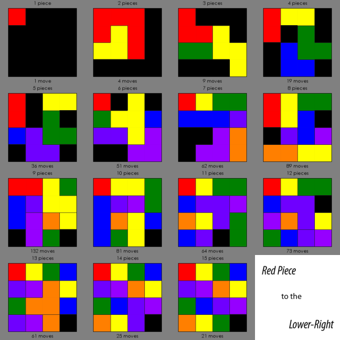
Running SBPSearcher on all the 4x4s takes about 3 hours (processing 12295564 puzzles), which was quite useful for fixing hidden bugs in the search algorithm. Here are the best simple^3 4×4 n-piece SBPs, where n goes from 1 to 15:

Click to view in full size

And for comparison, the move counts vs. the previously reported move counts:

   1   4   9  19  36  51  62  89 132  81  64  73  61  25  21
   1   4   9  24  36  52  68  90 132  81  64  73  61  25  21

    Notice that all the entries in the top row of the table are either less than or equal to their respective entry in the bottom row of the table, some (such as in the case of p=7 or p=4) being much less. This is because the previous search (run, in fact, as a subfeature in the sliding block puzzle evolver) started with all possible positions and defined the goal piece to be the first piece encountered going left to right, top to bottom, across the board. As such, the search included both all the 4×4 simple^3 sliding block puzzles as well as a peculiar subclass of sliding block puzzles where the upper-left square is empty but the goal piece is often a single square away! This accounts for the 6-piece case and the 8-piece case (in which the first move is to move the goal piece to the upper-left), but what about  the other two cases?

    For the 4-piece case, the originally reported puzzle (see here for the whole list) wasn’t simple^3, and it isn’t possible to convert it into a simple^3 SBP by shifting blocks in less than 5 moves. Interestingly, the new ‘best’ puzzle for 4 pieces is just James Stephens’ Simplicity with a few blocks shifted, a different goal piece, and a different goal position! (There could be copyright issues, so unless stated, the puzzles in this article are public domain except for the one in the upper-right corner of this image) Additionally, the 7-piece 68-move puzzle in the previous article is impossible to solve! The upper-left triomino should be flipped vertically in place. I expect this to have been a typing error, but the question still stands: Why is there a 6-move difference?

    As mentioned before, the actual stating of what constitutes a simple simple simple puzzle is as such: “A sliding block puzzle where the piece to be moved to the goal is in the upper-left corner, and the goal is to move the goal piece to the lower-right corner of the board”. Unfortunately, there’s some ambiguity as to when a piece is in the lower-right corner of the board – is it when the lower-right cell is taken up by a cell in the goal piece, or is it when the goal piece is as far to the lower-right as it can be? If we take the latter to be the definition, then additional ambiguities pop up when faced with certain problems, such as the following one often encountered by SBPSearcher:

Which piece has just moved into the lower-right?

Because of problems like these, SBPSearcher uses the former definition, which means that puzzles where the goal piece takes the shape of an R aren’t processed. (In actuality, it’s SBPFinder that does this checking, when it checks if a puzzle is in the ‘justsolved’ state). If we say that the first definition is stricter than the second, then it could be said that SBPSearcher searched only through the “Strict simple simple simple 4×4 Sliding Block Puzzles”. While I don’t think that any of the results would change other than the p=7 case, it would probably be worth it to modify a version of SBPSearcher so that it works with non-strict simple simple simple sliding block puzzles.

A few last interesting things: The 13-piece case appears to be almost exactly the same as the Time puzzle, listed in Hordern’s book as D50-59! (See also its entry in Rob Stegmann’s collection) Additionally, the same split-a-piece-and-rearrange-the-pieces-gives-you-extra-moves effect is still present, if only because of the chosen metric.

The Algorithm, In Slightly More Detail Than Last Time

There are only two ‘neat’ algorithms contained in the entire SBP collection of programs, these two in SBPFinder and SBPSearcher respectively. The first of them is used to find all possible sliding block puzzle ‘justsolved’ positions that fit in an NxM grid, and runs in at most O(2*3^(N+M-2)*4^((N-1)*(M-1))) time. (Empirical guess; Due to the nature of the algorithm, the calculation of the running time is probably very hairy).

First of all, the grid is numbered like this:

 0  1  3  6 10
 2  4  7 11 15
 5  8 12 16 19
 9 13 17 20 22
14 18 21 23 24

where the numbers increase going from top-right to lower-left, and moving to the next column over every time the path hits the left or bottom edges. (Technical note: For square grids, the formula x+y<N?TriangleNumber(x + y + 1) – x- 1:N*M – TriangleNumber(N + M- x – y – 1) + N – x – 1 should generate this array)

Then, the algorithm starts at cell #0, and does the following:

Given a partially filled board: (at cell 0 this board is all holes)

1. Take all the values of the cells from (cell_number-1) to the number of the cell to the left of me, and put that in list A.
2. Remove all duplicates from A.
3. If the following values do not exist in A, add them:  0 (aka a hole) and the smallest value between 1 and 4 inclusive that does not exist in A (if there is no smallest value between 1 and 4, don’t add anything except the 0)
4. Run fillboard (that is, the current function), giving it cell_number+1 and the board given to this level of the function with the value of cell_number changed to n, for each value n in A.

However, if the board is all filled (i.e, cell_number=25) , check to see that the board has holes and that it is justsolved, and if so, standardize the piece numbering and make sure that you haven’t encountered it before, and if so, sort the board into the appropriate piece number “box”.

Once the fillboard algorithm finishes, you should have N*M-1 boxes with all the possible justsolved positions that can be made on an N*M grid! There are a number of other possible methods that do the same thing- all it basically needs to do is generate all possible ways that pieces fitting in an NxM grid can be placed in a grid of the same size.

For example, you could potentially go through all possible 5-colorings of the grid (4-colors and holes), and remove duplicates, but that would take O(5^(N*M)) time, which isn’t the most feasible option for even a 4×4 grid.  You could also proceed in a way that would generate the results for the next number of pieces based on the results of the current number of pieces and all possible rotations and positions of a single piece in an NxM grid by seeing which pieces can be added to the results of the current stage, but that would take O(single_piece_results*all_justsolved_results). While that number may seem small, taking into account the actual numbers for a 4×4 grid (single_piece_results=11505 and all_justsolved_results=12295564) reveals the expected running time to be about the same as the slow 5-coloring method. However, it may be possible to speed up this method using various tricks of reducing which pieces need to be checked as to if they can be added. Lastly, one could go through all possibilities of edges separating pieces, and then figuring out which shapes are holes. The time for this would be somewhere between O(2^(3NM-N-M)) and O(2^(2NM-N-M)), the first being clearly infeasible and the second being much too plausible for a 4×4 grid.

In practice, the fillboard algorithm needs to check about 1.5 times the estimated number of boards to make sure it hasn’t found them before, resulting in about half a billion hash table lookups for a 4×4 grid.

The second algorithm, which SBPSearcher is almost completely composed of, is much simpler! Starting from a list of all justsolved puzzles (which can be generated by the fillboard algorithm), the following is run for each board in the list:

1. Run a diameter search from the current puzzle to find which other positions in the current puzzle’s graph have the goal piece in the same position;
2. Remove the results from step 1 from the list;
3. Run another diameter search from all the positions from step 1 (i.e consider all positions from step 1 to be 0 moves away from the start and work from there), and return the last position found where the goal piece is in the upper-left.

Step 2 is really where the speedup happens- Because each puzzle has a graph of positions that can be reached from it, and some of these positions are also in the big list of puzzles to be processed, you can find the puzzle furthest away from any of the goal positions by just searching away from them. Then, because the entire group has been solved, you don’t need to solve the group again for each of the other goal positions in it and those can be removed from the list. For a 4×4 board, the search can be done in 3 hours, 27 minutes on one thread on a computer with a Core I7-2600 @3.4 Ghz and a reasonable amount of memory. In total, the entire thing, finding puzzles and searching through all of the results, can be done in about 4 hours.

Of course, where there are algorithms, there are also problems that mess up the algorithms- for example, how would it be possible to modify SBPSearcher’s algorithm to do, say, simple simple puzzles? Or, is it possible to have the fillboard algorithm work with boards with internal walls or boards in weird shapes, or does it need to choose where the walls are? An interesting thing that would seem to point that the answer to the first question might be yes is that to find the pair of points furthest apart in a graph (which would be equivalent to finding the hardest compound SBP in a graph) requires only 2 diameter searches! Basically, you start with any point in the graph, then find the point furthest away from that, and let it be your new point. Then, find the point furthest away from your new point, and the two points, the one you’ve just found and the one before that, are the two points farthest away from each other. (See “Wennmacker’s Gadget”, page 98-99 and 7 in Ivan Moscovich’s “The Monty Hall Problem and Other Puzzles”)

Metrics

a.k.a. redefining the problem

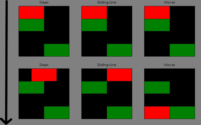
Through the last 3 posts on sliding block puzzles, I have usually used the “Moves” metric for defining how hard a puzzle is. Just to be clear, an action in the Moves metric is defined as sliding a single piece to another location by a sequence of steps to the left, right, up and down, making sure not to pass through any other pieces or invoke any other quantum phenomena along the way. (The jury is out as to if sliding at the speed of light is allowed). While the majority of solvers use the Moves metric (my SBPSolver, Jimslide, KlotskiSolver, etc.), there are many other metrics for giving an approximation to the difficulty of a sliding block puzzle, such as the Steps metric, and the not-widely used sliding-line metric. The Steps metric is defined as just that- an action (or ‘step’) is sliding a single piece a single unit up, down, left, or right. The sliding-line metric is similar: an action is sliding a single piece any distance in a straight line up, down, left or right. So far as I know, only Analogbit’s online solver and the earliest version of my SBPSolver used the steps metric, and only Donald Knuth’s “SLIDING” program has support for the sliding-line metric. (It also has support for all the kinds of metric presented in this post except for the BB metrics!)

Demonstration of various metrics

Additionally, each of the 3 metrics described above has another version which has the same constraints but can move multiple pieces at a time in the same direction(s). For example, a ‘supermove’ version of the Steps metric would allow you to slide any set of pieces one square in any one direction. (As far as I know, only Donald Knuth’s SLIDING program and Soft Qui Peut’s SBPSolver have support for any of the supermove metrics) In total, combining the supermove metrics with the normal metrics, there are 6 different metrics and thus 6 different ways to express the difficulty of a puzzle as a number. Note however, that a difficulty in one metric can’t be converted into another, which means that for completeness when presenting results you need to solve each sliding block puzzle 6 different ways! Even worse, the solving paths in different metrics need not be the same!

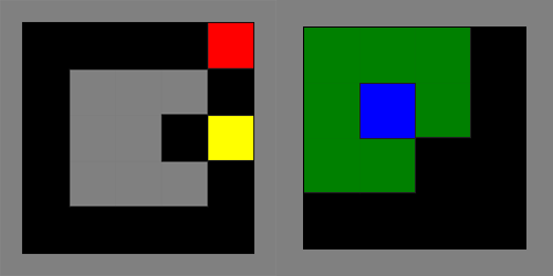
For example, in the left part of the image above, where the goal is to get the red piece to the lower-right corner, the Moves metric would report 1, and the red piece would go around the left side of the large block in the center. However, the Steps metric would report 5, by moving the yellow block left and then the red block down 4 times. Also, in the right picture both the Moves and Steps metrics would report ∞, because the green block can’t be moved without intersecting with the blue, and the blue block can’t be moved without intersecting with the green, but any of the Supermove metrics would report a finite number by moving both blocks at once!

Various other metrics can be proposed, some with other restrictions (You may not move a 1×1 next to a triomino, etc.), some which, like the Supermove metrics and the second puzzle above, actually change the way the pieces move, and you can eventually get to the point where it’s hard to call the puzzle a sliding block puzzle anymore. (For example, Dries de Clerq’s “Flying Block Puzzles” can be written as a metric: “An action is defined as a move or rotation of one piece to another location. Pieces may pass through each other while moving, but only one piece may be moved at a time”.

Suppose, however, that for now we’re purist and only allow metrics which generate numbers based on the step, sliding-line, moves, super-step, super-sliding-line, and super-moves metrics. It can be seen , quite obviously in fact, that these metrics don’t in all cases show the actual difficulty of the puzzle being considered. For example, take a very large (say 128×128) grid, and add a 126×126 wall in the center. Fill the moat that forms with 507 1×1 cells, all different pieces, and make the problem be to bring the block in the upper-left down to the lower-right. If my calculations are correct, the resulting problem should take 254*507+254=129,032 steps, sliding-line actions, and moves to solve, which would seem to indicate that this is a very hard puzzle indeed! However, any person who knows the first thing about sliding block puzzles should be able to solve it -assuming they can stay awake the full 17 hours it would take!

Because of this discouraging fact- that is, 6 competing standards, none of which are quite right, I would like to introduce a 7th, this one based on a theoretical simulation of a robot that knows the first thing about sliding block puzzles, but nothing else.

The BB Metric

a.k.a. attempting not to invoke the xkcd reference

Nick Baxter and I have been working on a metric which should better approximate the difficulty of getting from one point to another in a position graph. The basic idea is that the difficulty of getting from node A to node B in a graph is about the same as the average difficulty of getting from node A to node B in all spanning trees of the graph. However, finding the difficulty of getting to node A to node B in a tree is nontrivial, or at least so it would seem at first glance.

Suppose you’re at the entrance of a maze, and the maze goes on for far enough and is tall enough such that you can only see the paths immediately leading off from where you are. If you know that the maze is a tree (i.e, it has no loops), then a reasonable method might be to choose a random pathway, and traverse that part of the maze. If you return from that part to the original node, then that part doesn’t contain the goal node and you can choose another random pathway to traverse, making sure of course not to go down the same paths you’ve gone down before. (Note that to be sure that the goal node isn’t in a part of the maze, you need to go down all the paths twice, to walk down a path and then back up the path). For now, we take the difficulty of the maze to be the average number of paths you’ll need to walk on to get to the goal node or decide that the maze has no goal(counting paths you walk down and up on as +2 to the difficulty). Because of the fact that if the node you’re in has no descendant nodes which are the goal node you’ll need to go down all of the paths leading from that node twice, the difficulty of the part of the maze tree branching off from a node A can be calculated as

sum(a_i+2,i=1 to n)     (eq. 1)

where n is the number of subnodes, and a_i is the difficulty of the ith subnode. Also, if the node A is on the solution path between the start and end nodes, then the difficulty of A can be calculated as

a_n+1+1/2 sum(a_i+2,i=1 to n-1)    (eq. 2)

where a_n is assumed to be the subnode which leads to the goal. This basically states that on average that you’ll have to go down half of the subpaths and the path leading to the goal to get to the goal. Because root nodes are assumed to have 0 difficulty, you can work up from the bottom of the maze, filling in difficulties of nodes as you go up the tree. After the difficulty of the root node has been calculated, the length of the path between start and end nodes should be subtracted to give labyrinths (mazes with only a single path) a BB difficulty of 0.

Perhaps surprisingly, it turns out that using this scheme, the difficulty of a tree with one goal node is always measured as V-1-m, where V is the number of nodes in the tree (and V-1 is the number of edges, but this is not true for graphs) and m is the number of steps needed to get from the start node to the end node in the tree! Because of this, the difficulty of getting from one point to another in a graph under the BB metric is just the number of vertices, minus one, minus the average path length between the start and end nodes in the graph.

A few things to note (and a disclaimer): First of all, the actual graph of which positions can be reached in 1 action from each of the other positions actually depends on the type of move chosen, so the BB metric doesn’t really remedy the problem of the 6 competing standards! Secondly, the problem of computing the average path length between two points in a graph is really really hard to do quickly, especially because an algorithm which would also give you the maximum path length between two points in polynomial time would allow you to test if a graph has a Hamiltonian Path in polynomial time, and since the Hamiltonian Path problem is NP-Complete, you could also do the Traveling Salesman Problem, Knapsack Problem, Graph Coloring Problem, etc. in polynomial time! Lastly, I haven’t tested this metric on any actual puzzles yet, and I’m also not certain that nobody else has come up with the same difficulty metric. If anybody knows, please tell me!

One last note: Humans don’t actually walk down mazes by choosing random paths- usually it’s possible to see if a path dead-ends, and often people choose the path leading closest to the finish first, as well as a whole host of other techniques that people use when trying to escape from a maze. Walter D. Pullen, author of the excellent maze-making program Daedalus, has a big long list of things that make a maze difficult here. (Many of these factors could be implemented by just adding weights to eqns. 1 and 2 above)

Open Problems

a.k.a. things for an idling programmer to do

• What are the hardest simple simple simple 3×4 sliding block puzzles in different metrics? 2×8? 4×5? (Many, many popular sliding block puzzles fit in a 4×5 grid)
• How much of a difference do the hardest strict simple^3 puzzles have with the hardest simple^3 SBPs?
• How hard is it to search through all simple simple 4×4 SBPs? What about simple SBPs?
• (Robert Smith) Is there any importance to the dual of the graph induced by an SBP?
• Why hasn’t anybody found the hardest 15 puzzle position yet? (According to Karlemo and Östergård, only 1.3 TB would be required, which many large external hard drives today can hold! Unfortunately, there would be a lot of reading and writing to the hard disk, which would slow down the computation a bit.) (Or have they?)
• Why 132?
• What’s the hardest 2-piece simple sliding block puzzle in a square grid? Ziegler-Hunts & Ziegler-Hunts have shown a lower bound of 4n-16 for an nxn grid, n>6. How to do so isn’t too difficult, and is left as a puzzle for the reader.
• Is there a better metric for difficulty than the BB metric?
• Is there a better way to find different sliding block puzzle positions? (i.e, improve the fillboard algorithm?)
• Is it possible to tell if a SBP is solvable without searching through all possible positions? (This question was proposed in Martin Gardner’s article on Sliding Block Puzzles in the February 1964 issue of Scientific American)
• (Robert Smith) How do solutions of SBPs vary when we make an atomic change to the puzzle?
• Are 3-dimensional sliding block puzzles interesting?
• Would it be worthwhile to create an online database of sliding block puzzles based on the OEIS and as a sort of spiritual successor to Edward Hordern’s Sliding Piece Puzzles?

Sources

Ed Pegg, “Math Games: sliding-block Puzzles”, http://www.maa.org/editorial/mathgames/mathgames_12_13_04.html

James Stephens, “Sliding Block Puzzles”, http://puzzlebeast.com/slidingblock/index.html (see also the entire website)

Rob Stegmann, “Rob’s Puzzle Page: Sliding Puzzles”, http://www.robspuzzlepage.com/sliding.htm

Dries De Clerq, “Sliding Block Puzzles” http://puzzles.net23.net/

Neil Bickford, “SbpUtilities”, http://github.com/Nbickford/SbpUtilities

Jim Leonard, “JimSlide”, http://xuth.net/jimslide/

The Mysterious Tim of Analogbit, “Sliding Block Puzzle Solver”, http://analogbit.com/software/puzzletools

Walter D. Pullen, “Think Labyrinth!”, http://www.astrolog.org/labyrnth.htm

Donald Knuth, “SLIDING”, http://www-cs-staff.stanford.edu/~uno/programs/sliding.w

Martin Gardner, “The hypnotic fascination of sliding-block puzzles”, Scientific American, 210:122-130, 1964.

L.E. Hordern, “Sliding Piece Puzzles”, published 1986 Oxford University Press

Ivan Moscovich, “The Monty Hall Problem and Other Puzzles”

R.W. Karlemo, R. J. Östergård, “On Sliding Block Puzzles”, http://citeseerx.ist.psu.edu/viewdoc/summary?doi=10.1.1.55.7558

Robert Hearn, “Games, Puzzles, and Computation”, http://groups.csail.mit.edu/mac/users/bob/hearn-thesis-final.pdf

Ruben Grønning Spaans, “Improving sliding-block puzzle solvingusing meta-level reasoning”, http://daim.idi.ntnu.no/masteroppgave?id=5516

John Tromp and Rudi Cilibrasi, “”Limits on Rush Hour Logic Complexity”, arxiv.org/pdf/cs/0502068

David Singmaster et al.,  “Sliding Block Circular”, www.g4g4.com/pMyCD5/PUZZLES/SLIDING/SLIDE1.DOC

Thinkfun & Mark Engelberg, “The Inside Story of How We Created 2500 Great Rush Hour Challenges”, http://www.thinkfun.com/microsite/rushhour/creating2500challenges

Ghaith Tarawneh, “Rush Hour [Game AI]”, http://black-extruder.net/blog/rush-hour-game-ai.htm

Any answers to questions or rebukes of the data? Post a comment or email the author at (rot13) grpuvr314@tznvy.pbz